July 20, 2024 by Cyril Noirot
Determinant and effects of supply and demand: the Fulton Fish Market
The Fulton Fish Market, a key part of NYC’s trade for over 150 years, offers insights into market dynamics, price elasticity, and economic behavior. This blog is an attempt to reproduce and explain Graddy’s work on imperfect competition, price discrimination, and weather’s impact using Python-based analysis.
Dataset overview and methodology
The dataset
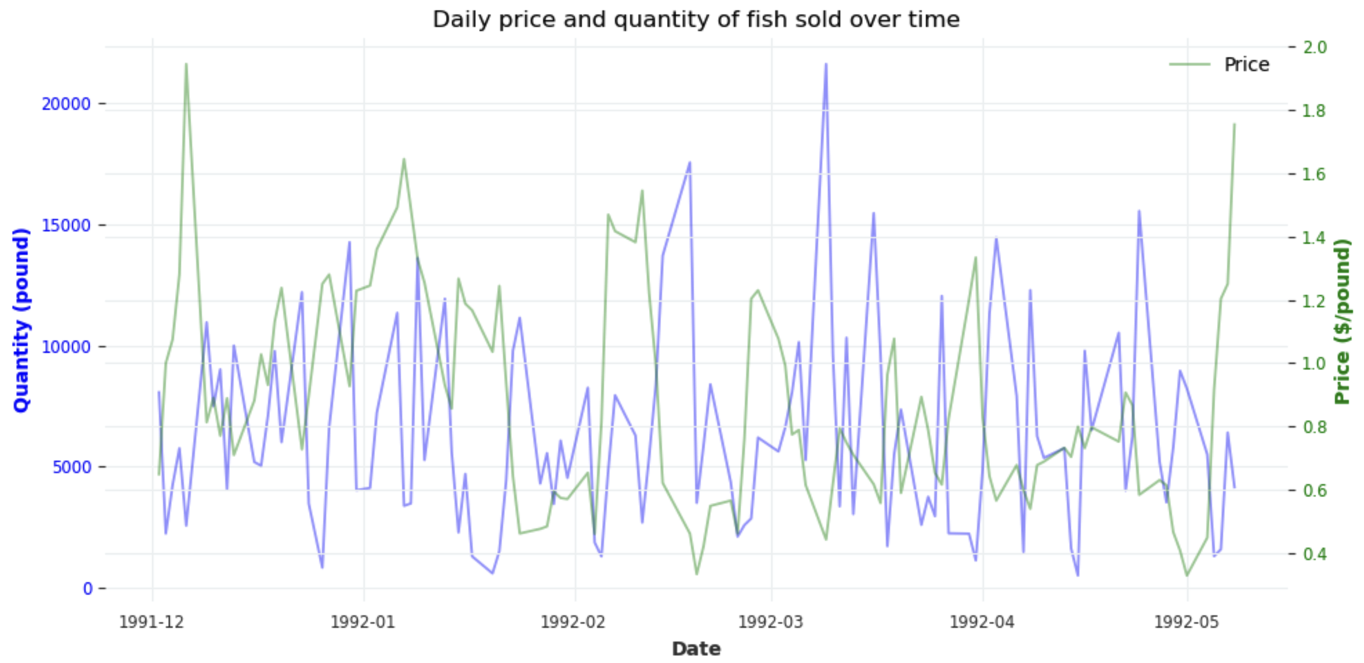
Dataset consists of whiting transactions between late 1991 and early 1992, including:
- Quantity: total amount sold on a day in pounds
- Price: average price per pound for the day
- Weather data (wind speeds and wave heights as proxies for supply shocks).
- Buyer demographics: Asian or White.
EDA: price and quantity response to weather
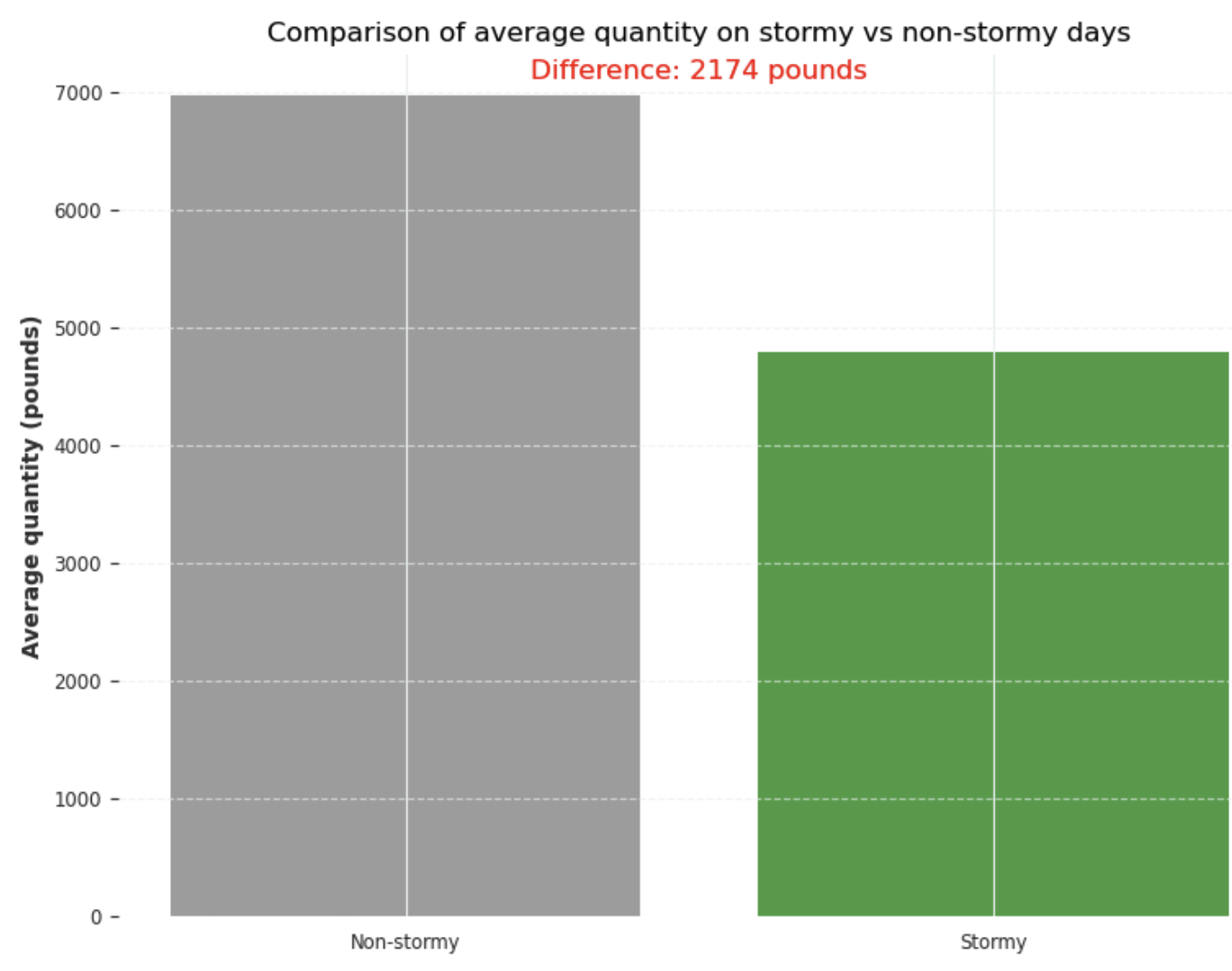
The average quantity on a clear day was 2,371 pounds more than on a stormy day.
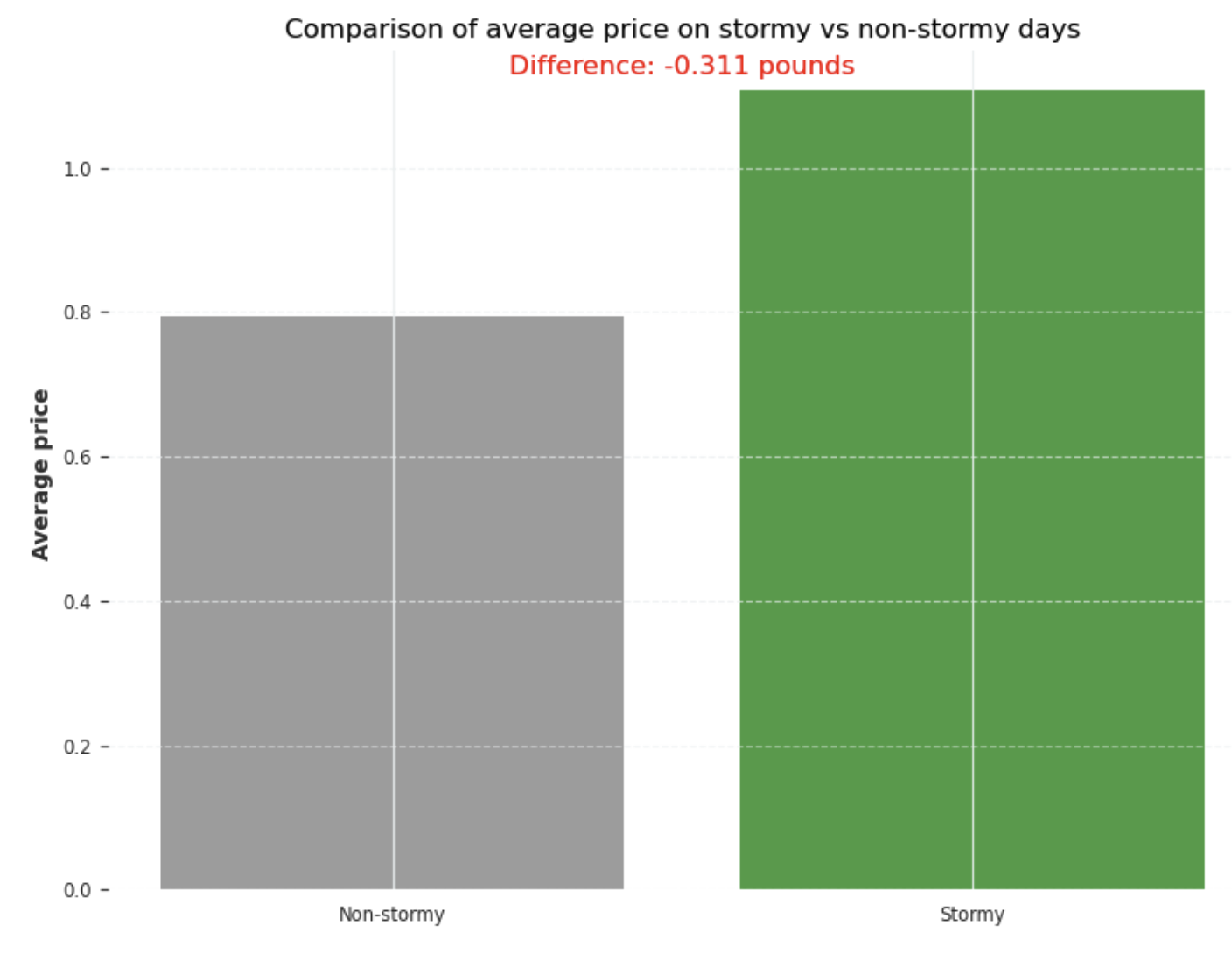
The average price on a clear day was 32 cents per pounds less than on a stormy day.
Price elasticity estimate
Definition
Price elasticity of demand (PED) $\varepsilon$ measures how responsive the quantity demanded ( Q ) is to changes in price (P):
$$ \varepsilon = \frac{\text{change in quantity demanded}}{\text{change in price}} $$
- If |$\varepsilon$| > 1 (elastic demand), quantity demanded is highly responsive to price changes.
- If |$\varepsilon$| < 1 (inelastic demand), quantity demanded is less responsive to price changes.
In a log-log model, the beta coefficient ($\beta_{\ln(\text{price})}$) represents the elasticity of the target variable with respect to the predictor. The model assumes that the relationship between variables, such as price and quantity demanded, is linear. In other words, the percentage change in one variable is proportional to the percentage change in another variable when both are expressed as logarithms.
The model is specified by the equation below:
$$ \ln(\text{qty}) = \beta_0 + \beta_1 \cdot \ln(\text{price}) + \beta_2 \cdot \ln(\text{price}) \times \text{stormy} +\beta_3 \cdot x$$
- where x are exogenous dummy variables representing days of the week and the weather onshore.
As display before the stormy conditions significantly impact the quantity sold and the average price. Therefore we introduce a interaction term so the total effect of price is context-dependent:
- Elasticity for non-stormy days: $\beta_1$
- Elasticity for stormy days: $\beta_1 + \beta_2$
Model fitting
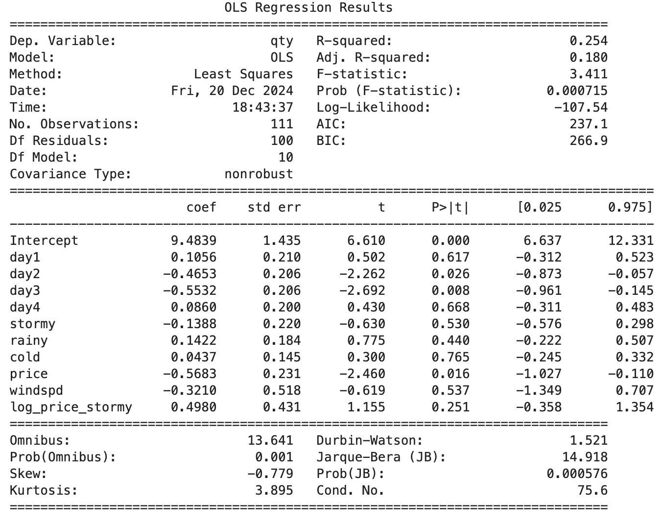
Despite a low R^2 , we will proceed with analyzing the impact of price. However, in a real business scenario, it is crucial to establish clear performance benchmarks for the model, such as achieving an R^2 of at least 0.8, before relying on its insights for decision-making.
Model diagnostics
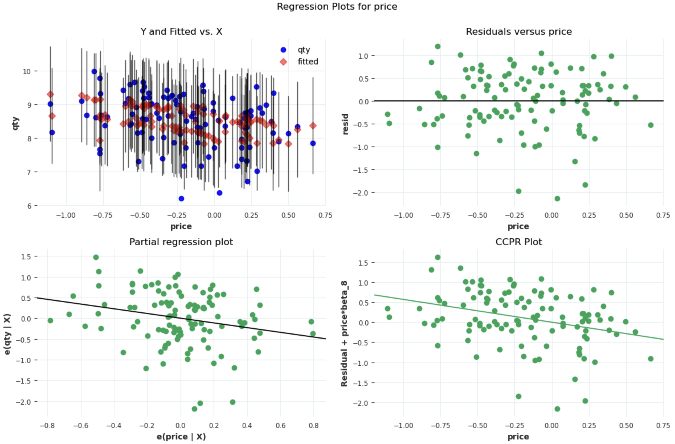
The partial regression plot shows a negative relationship between price and quantity (log-log elasticity of -0.5683). As price increases, quantity decreases, highlighting the inverse relationship dictated by the law of demand: ‘a 1% increase in price leads to a 0.5683% decrease in quantity on non-stormy days.’
The CCPR plot reinforces this trend by illustrating the direct contribution of price to the dependent variable. The negative slope confirms that higher prices result in lower quantities, even after accounting for residuals and other factors.
Interpretation
The low negative price elasticity reveals that demand is inelastic, meaning a percentage increase in price leads to a smaller percentage decrease in quantity. This suggests buyers are relatively insensitive to price changes under normal conditions.
The interaction between stormy weather and price significantly modifies the elasticity of demand, reducing the steepness of the quantity decline. Stormy conditions likely create supply shortages or urgency among buyers, making them less sensitive to price changes.
References
Graddy, K., & Hall, G. (2010). A dynamic model of price discrimination and inventory management at the Fulton Fish Market. Journal of Economic Behavior & Organization, 80(1), 6–19. https://doi.org/10.1016/j.jebo.2010.08.018